Empowering Safe Reinforcement Learning for Power System Control with CommonPower

Authors:

• Hannah Markgraf, Technical University of Munich, hannah.markgraf@tum.de

• Michael Eichelbeck, Technical University of Munich, michael.eichelbeck@tum.de

• Matthias Althoff, Technical University of Munich, althoff@in.tum.de

This tutorial introduces the CommonPower library, designed to benchmark safe reinforcement learning (RL) algorithms on control problems for power systems. We highlight two crucial issues in RL for power system control: safeguarding RL decision-making and assessing the impact of forecast quality on control performance. Participants will learn how to use CommonPower to further invesitigate these topics.

Table of Contents

• Overview

• Climate Impact

• Target Audience

• Background & Prerequisites

• Software Requirements

• Data Description

• Part 1: Modular Power System Modeling with CommonPower

• Part 2: Safe Reinforcement Learning for Power System Control

• Part 3: More Advanced Capabilities of CommonPower

• Results & Discussion

• References

## Overview

This tutorial provides all necessary basics for benchmarking safe RL controllers on power system control tasks using CommonPower. A special focus lies on assessing the impact of forecast accuracy on controller performance. We first provide some theoretical background on the necessity and the mechanisms of safeguarding RL. Then, we introduce how to set up a power system control problem in CommonPower and solve it using the built-in model-predictive controller (MPC). The second part explains how CommonPower safeguards RL and provides hands-on experience in training a safe RL agent. We show the impact of the choice of forecasting method on the performance of both the MPC and the RL controller. In the third part, we introduce more advanced capabilities of CommonPower, like importing grid topologies from pandapower or modeling new components.

🎯 The user of this notebook will:

• Familiarize themselves with the modular approach of CommonPower for modeling power systems,

• Learn how to benchmark RL agents against an MPC baseline using CommonPower,

• Understand the importance of safeguarding vanilla RL algorithms, in particular when solving safety-critical tasks, such as operating power systems, and

• Assess the impact of using flawed forecasts on control performance.

Climate Impact

Since decision making in power system control is highly dependent on forecasts of several quantities, such as electric loads, renewable generation, and electricity prices, controllers based on RL emerge as a promising solution: Using neural networks as function approximators for detecting complex patterns in large amounts of data, they have the potential of outperforming traditional control approaches, such as MPC. To systematically compare different solution approaches, benchmarks are required. Our CommonPower library provides a modular framework for composing benchmarks and integrating different forecasting strategies to assess the impact of prediction accuracy on the performance of controllers. Furthermore, CommonPower addresses a central issue that hinders the applicability of RL in real-word settings: the challenge of incorporating physical constraints of the power system into the RL algorithm.

Our goal is to motivate other researchers to create meaningful benchmarks, develop more powerful safe RL algorithms, and assess the impact of forecast accuracy on their performance, ultimately improving our understanding of the interplay of RL algorithms and safeguarding mechanisms. In essence, our workshop serves as a catalyst for transformative advancements in RL for power system control, accelerating its adoption in real-world applications.

Target Audience

This tutorial is designed for:

1. Researchers and companies working on RL for diverse power system control tasks

2. Researchers and companies working on forecasting techniques (renewable generation, household loads, electric vehicle consumption patterns,…) that would like to test the impact of their models on the performance of different control strategies, including RL controllers

Background & Prerequisites

Prerequisites

This tutorial requires beginner level in Python or another high-level scripting language. Furthermore, a solid understanding of RL algorithms is useful, but not necessary. We highly recommend the OpenAI SpinningUp guide for an introduction to deep RL.

In the following, we will give a short introduction to RL for power system control and how to safeguard decisions made by RL controllers.

Reinforcement Learning for Power System Control

Problem Statement: Power System Control

The primary application areas of CommonPower are smart home energy management, demand response, and economic dispatch in microgrids. We model these control tasks as discrete-time receding-horizon optimal control problems. Within a network, we assume a set of nodes \(\mathcal{N}\). A node can either be a prosumer or a balancing asset. The set of all prosumers \(\mathcal{P} \subseteq \mathcal{N}\) is what we consider to be actively controllable. A set of balancing assets \(\mathcal{A} = \mathcal{N} \setminus \mathcal{P}\) represents assets that are utilized by the grid operator to establish grid stability. Prosumers can form disjoint coalitions \(\mathcal{G}^i \subseteq \mathcal{P}\), \(\bigcap_i \mathcal{G}^i = \emptyset\), \(\bigcup_i \mathcal{G}^i = \mathcal{P}\) in which all members are jointly controlled. We refer to centralized control for the special case in which there are no balancing assets, and all prosumers are controlled centrally, i.e., there is only one coalition \(\mathcal{G} = \mathcal{P} = \mathcal{N}\). In every coalition \(i\),

• \(u_t^i\) is the vector of controllable inputs,

• \(d_t^i\) is the vector of uncontrollable exogenous inputs,

• \(\hat{d}_t^i\) is the vector of possibly inaccurate forecasts for \(d_t^i\),

• \(x_t^i\) is the state vector,

• \(h^i(x_t^i, \hat{d}_t^i)\) describes the input coupling, i.e., constraints arising from power flow or power balance considerations,

• \(f^i(x_t^i, \hat{d}_t^i, u_t^i)\) models the system dynamics, and

• \(C^i(x_t^i, \hat{d}_t^i, u_t^i)\) is the cost function.

Inputs and states are restricted by constant technical limits \([\underline{u}^i, \overline{u}^i]\) and \([\underline{x}^i, \overline{x}^i]\), respectively. For every time step \(t\), each coalition \(i\) solves for a control horizon \(T\) the optimization problem

:nbsphinx-math:`begin{align}

& min_{u^i} sum_{t=0}^T C^i(x_t^i, hat{d}_t^i, u_t^i) tag{1a}\ & s.t. nonumber tag{1b}\

& u_t^i in [underline{u}^i, overline{u}^i] \ & u_t^i = h^i(x_t^i, hat{d}_t^i) \ & x_t^i in [underline{x}^i, overline{x}^i] \ & x_{t+1}^i = f^i(x_t^i, hat{d}_t^i, u_t^i).

end{align}`

In the case of centralized control, all nodes and their input coupling are contained in (1b), resulting in a dispatch solution that satisfies all system constraints.

In decentral control, (1b) only contains input coupling constraints within coalitions, but not between them, since we assume that coalitions do not communicate with each other. This makes it very unlikely that the independent dispatch decisions of all coalitions fulfill the input coupling constraint on the network level. Therefore, in practice, we always model at least one balancing asset in decentral control.

Balancing assets are dispatched as a second stage by solving (1) with a single coalition \(i = \mathcal{A}\). Here, the previously computed input trajectories for all coalitions are concatenated in \(u^{\mathcal{P}}\), which is treated as uncontrollable input. The input coupling constraint is then given by \(u_t^{\mathcal{A}} = h^{\mathcal{A}}(x_t^{\mathcal{A}}, \begin{bmatrix} \hat{d}^{\mathcal{A}} & u_t^{\mathcal{P}} \end{bmatrix}^{\top})\).

Solving the Power System Control Problem Using Reinforcement Learning

The problem statement in (1) can be considered for both the central and decentral case as a sequential decision-making process under uncertainty. RL is the standard machine learning (ML) approach for solving such problems. The core concept underlying RL is to learn by trial and error, or through repeated experimentation. An RL agent finds a good strategy by repeatedly interacting with an environment. In each step of the interaction, the agent will make a decision based on an observation of the state of the environment. It will then receive a reward that expresses how good or bad that decision was. Training an RL agent refers to adjusting the strategy of the agent with the goal of achieving higher rewards.

This concept is visualized in the figure below. Imagine a dog trying to learn to grab a stick. The dog is the agent, and the human throwing the stick is the environment. Each time the dog observes the human throwing the stick, it will perform an action like jumping or running. If it manages to catch the stick, it will receive a reward in the form of a cookie from the human. Eventually, the dog will learn a strategy that yields the highest reward.

Compared to classic control approaches, such as optimal control, RL does not require an explicit definition of the system dynamics \(f\). Instead, implicit knowledge about \(f\) is gathered through interaction with the system.

Decentral control of a system with multiple agents can be realized using multi-agent reinforcement learning (MARL). In MARL, the underlying control problem is commonly modeled as a partially observable Markov game (POMG). It is defined as a tuple \((\mathcal{L}, \mathcal{S}, (\mathcal{U}^i, \mathcal{O}^i, R^i)_{\forall i \in \mathcal{L}}, T, \gamma)\) (Yu et al., 2022), where

• \(\mathcal{L} = \{1,...,L\}\) is the set of agents,

• \(\mathcal{S} := [\underline{s}, \overline{s}]\) is the global state space of the environment,

• \(\mathcal{O}^i := [\underline{o}^i, \overline{o}^i]\) is the observation space of an agent,

• \(\mathcal{U}^i :=[\underline{u}^i, \overline{u}^i]\) is the input space (also referred to as the action space) of an agent,

• \(R^i: \mathcal{O}^i \times \mathcal{U}^i \rightarrow \mathbb{R}\) is the agent-specific reward function,

• \(T: \mathcal{S} \times \mathcal{U}_1 \times ... \times \mathcal{U}_L \times \mathcal{S} \rightarrow \mathbb{R}\) is the probability density function modeling state transitions, and

• \(\gamma \in [0,1)\) is the discount factor used to weigh future rewards.

Note that we use the notation \((\mathcal{U}^i, \mathcal{O}^i, R^i)_{\forall i \in \mathcal{L}}\) to refer to the tuple of individual quantities \(\left(\mathcal{U}_1,...,\mathcal{U}_L, \mathcal{O}_1,...,\mathcal{O}_L, R_1,...,R_L\right)\). Centralized RL control is a special case of the POMG with \(L=1\), resulting in a Markov decision process (MDP).

Even though the presented POMG does not model exactly the same problem as (1), the two are closely related. During training, the RL agents learn the policy \(\pi^i\) with \(u^i_t~=~\pi^i(o^i_t)\) maximizing the expected cumulative discounted reward \(\mathbb{E}_{\pi^i}[\sum_{k=0}^{T} \gamma^k R^i_{t+k+1}]\) (Sutton et al., 2018). However, vanilla RL cannot consider the constraints (1b), except for the input limits, which are captured by the action space \(\mathcal{U}^i\). This is why we require a safety shield like the one implemented in CommonPower. Without any safety considerations, the reward is chosen as the negative stage cost \(R^i = -C^i\). In Part 2 we describe how to modify the reward function to incorporate information about any interventions of the safety shield. We choose the observation of an agent as the concatenation of its state variables and the forecasts of uncontrollable inputs \(o^i_t = \begin{bmatrix} x^i_t & \hat{d}^i_t \end{bmatrix}^T\).

### Safeguarding Reinforcement Learning

We can differentiate between different safety levels for control problems (Brunke et al., 2022):

• Safety level 1: constraint satisfaction encouraged,

• Safety level 2: constraint satisfaction with high probability, and

• Safety level 3: constraint satisfaction guaranteed.

For power system control, we want to achieve safety level 3 to avoid critical failures. The work by (Krasowski et al., 2022) summarizes this field of research under the term provably safe reinforcement learning. They identify three main approaches to achieve RL with guaranteed constraint satisfaction, namely action projection, action replacement, and action masking. Action masking is a pre-emptive method, meaning that the RL algorithm is modified in a way that only actions that fulfill all constraints can be selected. Both action replacement and projection are post-posed, meaning that any unsafe action selected by the RL agent will be modified such that it fulfills the constraints. It can either be replaced by some safe action – that is action replacement – or by the action that is closest to the unsafe action under a defined distance metric, e.g., Euclidian distance – this is termed action projection. The figure below visualizes the three concepts.

Figure 2: Overview of the main approaches in provably safe reinforcement learning. (a) and (b) highlight the differences between post-posed and pre-emptive shielding. The subfigures (c-e) show how a safe action is obtained from the available set of provably safe actions. Source: (Krasowski et al., 2023)

CommonPower currently focuses on action projection. In each time step, we obtain the safe action by solving a constrained optimization problem that minimizes the Euclidian distance between the proposed action \(u^i_t\) and the safe action. The constraints of the subsystem controlled by the RL agent can be extracted automatically, thanks to the symbolic modeling approach of CommonPower. The action projection problem solved by the safety shield results in :nbsphinx-math:`begin{align}

& tilde{u}_t^i = argmin_{u’} |u’ - u^i_t|_2\ & s.t. (1b)

end{align}`

When using post-posed safeguarding during RL training, the behavior policy used to gather data differs from the target policy that is learned. Normally, a policy is updated based on a batch of tuples \((o^i_t, u^i_t, o^i_{t+1}, r^i_t)\). When a correction of \(u^i_t\) becomes necessary, this tuple could be changed to \((o^i_t, \tilde{u}_t^i, o^i_{t+1}, r^i_t)\), which features the safe action and the reward obtained from applying this action. However, this would mean updating the policy with actions that do not stem from the most recent policy, which is an expected procedure for off-policy algorithms but can be problematic for on-policy algorithms (Krasowski et al., 2022). Instead, we use an adaption penalty \(\tilde{r}^i_t = R^i(o^i_t, u^i_t, o^i_{t+1})+R^i_{penalty}(u^i_t, \tilde{u}_t^i)\), such that the tuple used for learning is \((o^i_t, u^i_t, o^i_{t+1}, \tilde{r}^i_t)\). This penalty informs the agent about the intervention of the safety layer. How to compute the penalty is a design choice and can require careful tuning.

# Utils
import pathlib
from datetime import datetime, timedelta

# Data visualization
import matplotlib.pyplot as plt

# Reinforcement learning
from stable_baselines3 import PPO

# CommonPower
from commonpower.modeling import ModelHistory
from commonpower.core import System
from commonpower.models.buses import *
from commonpower.models.components import *
from commonpower.models.powerflow import *
from commonpower.control.controllers import RLControllerSB3, OptimalController
from commonpower.control.observation_handling import ObservationHandler
from commonpower.control.safety_layer.safety_layers import ActionProjectionSafetyLayer
from commonpower.control.safety_layer.penalties import DistanceDependingPenalty
from commonpower.control.runners import SingleAgentTrainer, DeploymentRunner
from commonpower.control.wrappers import SingleAgentWrapper
from commonpower.control.configs.algorithms import SB3MetaConfig, SB3PPOConfig
from commonpower.control.util import predicted_cost_callback
from commonpower.control.logging_utils.loggers import *
from commonpower.data_forecasting import *
from commonpower.modeling.param_initialization import *

# Load the TensorBoard notebook extension
%load_ext tensorboard

Data Description

CommonPower already contains some time series data of loads, renewable generation, spot market prices, etc. We will download the data we need into a new folder.

For the household load data as well as the renewable generation, we use time series provided by the SimBench benchmark data set. To make our case study more interesting, we use dynamic electricity prices. We employ the spot market prices from Energi Data Service from the year 2016 and scale them such that the mean price over the year matches the mean consumer electricity price per kWh in Germany.

Data Preprocessing

CommonPower offers different data sources (see documentation) to deal with various file extensions, for example csv files. We will use the CSVDataSource for the load and PV generation data as well as the electricity prices. The price for selling 1 kWh of electricity is assumed to be constant according to the “Einspeisevergütung” from 2016. Therefore, we use a ConstantDataSource.

current_path = pathlib.Path().absolute()
data_path = current_path / 'data' / 'data_ICLR'
data_path = data_path.resolve()

date_format = "%Y-%m-%d %H:%M:00"

# Data source (ds) for active power(p) of a household
p_load_ds = CSVDataSource(data_path / 'ICLR_load.csv',
            datetime_format=date_format,
            resample=timedelta(minutes=60))

# We neglect reactive power (q) during this tutorial
q_load_ds = ConstantDataSource({"q": 0.0}, date_range=p_load_ds.get_date_range(), frequency=timedelta(minutes=60))

# Data source for electricity prices
buying_price_ds = CSVDataSource(data_path / 'ICLR_prices.csv',
            datetime_format=date_format,
            resample=timedelta(minutes=60))

# Data source for selling prices of electricity
selling_price_ds = ConstantDataSource({"psis": 0.1197}, date_range=buying_price_ds.get_date_range(), frequency=timedelta(minutes=60))

# Data source for PV generation
pv_ds = CSVDataSource(data_path / 'ICLR_pv.csv',
        datetime_format=date_format,
        resample=timedelta(minutes=60)).apply_to_column("p", lambda x: -x)

While the data itself is stored in the so-called data sources, CommonPower also has data providers. A data provider is defined by a data source and a forecaster providing observations of the respective quantity, for example, forecasts of the electric load of a household. For simplicity, we will predict all quantities with historic values from the previous day using the PersistenceForecaster. To see other available forecasters, you can have a look at the documentation.

We define a forecast_horizon to specify how many time steps we want to look into the future. The forecast_frequency tells us the time interval between two forecasts.

forecast_frequency = timedelta(minutes=60)
forecast_length = 12  # [time steps] --> since frequency is one hour, this is 12h
forecast_horizon = timedelta(hours=forecast_length)

forecaster = PersistenceForecaster(frequency=forecast_frequency, horizon=forecast_horizon, look_back=timedelta(hours=24))

load_p_dp = DataProvider(p_load_ds, forecaster)  # [kW]
load_q_dp = DataProvider(q_load_ds, forecaster)  # [kVA]
price_dp = DataProvider(buying_price_ds, forecaster)  # [€]
selling_price_dp = DataProvider(selling_price_ds, forecaster)  # [€]
pv_dp = DataProvider(pv_ds, forecaster)  # [kW]

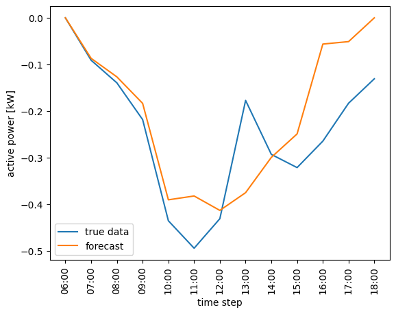
To show you what a forecast looks like, let us plot the true data and the observations of the data provider.

timestamps = pd.date_range(start=datetime(2016, 5, 12, 6), periods=forecast_length + 1, freq=forecast_frequency)

true_data = pv_ds(timestamps[0], timestamps[-1])
forecast = pv_dp.observe(timestamps[0])["p"]

plt.plot(true_data, label="true data")
plt.plot(forecast, label="forecast")
plt.xticks(range(len(true_data)), timestamps.strftime('%H:%M'), rotation=90)
plt.xlabel("time step")
plt.ylabel("active power [kW]")
plt.legend()
plt.show()

With all data sources set up, we can now dive into an example of how to model and control a power system in CommonPower.

Part 1: Modular Power System Modeling with CommonPower

This section covers the basics of CommonPower. We will learn how to model a power system in a modular fashion and simulate it using a built-in optimal controller. To provide maximum flexibility for modelling, CommonPower follows a modular approach. This means that there are different basic object classes, and you can build your custom classes on top of them. The most important classes are:

• System: This class is the unique “root” of the power system representation. It keeps a list of all nodes and lines in the system.

• Node: The superclass for busses and components. A Node can have subordinate child nodes. It can be controlled or uncontrolled – in the latter case, it will pull the time series of its characterists from a data source.

• Bus: Busses come with an internal power balance equation and sum the cost of their children.

• Component: Represents a specific electical device, e.g. battery, PV, gas generator, etc. Cannot have children. By implementing subclasses of components arbitrary devices can be realized.

• Line: Represents power transmission lines. Subclasses allow for flexible modelling in conjunction with corresponding power flow models.

• Power Flow: This defines how the power flow is modelled on the system level.

In this tutorial, we will only cover a few of these classes. We have chosen a simplified use case where we model a household with a battery storage system and a solar cell (PV). The battery and the PV are pre-defined components in CommonPower and you will learn how to configure such components. The ultimate goal is to then find a good control strategy for this system to keep the electricity cost as low as possible.

More advanced capabilities of CommonPower, such as modeling a power grid or creating new components, will be covered in Part 3 of the tutorial!

Modeling of power system entities

In CommonPower, every power system entity (power flow, busses, components) is described by a symbolic model. We use these models to compute optimal control actions or safety adjustments. The necessary optimization problems are automatically generated in the background and solved within the Python framework Pyomo. Pyomo defines models with variables, parameters, and constraints. We extend this classification to gain some nuance. In CommonPower, we use the following types of model elements:

• INPUT - Input variable.

• DATA - Exogenous input, which is read from a data provider.

• STATE - State variable.

• VAR - Generic variable. The difference to state variables is that VAR does not have to be initialized.

• CONSTANT - Fixed Parameter. Parameters can either be constant across runs or be initialized in each run based on a specific logic.

• COST - Cost variable. This is essentially a generic variable but explicitly defined to simplify downstream analysis.

• CONSTRAINT - Constraint. Input coupling and dynamics functions are defined with this type.

• SET - Set. Sets can be useful to specify the values a discrete variable can take.

These model elements are base of every model. We define dynamics and cost functions as constraints.

As a modeling example, let us have a closer look at a simple Component: ESSLinear, a linear model of an energy storage system.

class ESSLinear(Component):
  """
  Simplified ESS model without efficiencies and without cost function.
  """

  CLASS_INDEX = "el"  # This is used to name components in the pyomo model

  @classmethod
  def _get_model_elements(cls) -> List[ModelElement]:
    """
    Here we define all model elements except constraints.
    If not specified otherwise, all such elements are indexed, i.e., they are vectors covering the entire forecast horizon.
    This way, our symbolic model already represents a model-predictive control formulation.
    """

    model_elements = [
      # All element of type INPUT are automatically configured in controllers as control inputs.
      # When defining control inputs, the bounds defined in the component configuration during initialization are passed as well, e.g., establishing the RL action space.
      ModelElement("p", et.INPUT, "active power"),
      # Model elements of type VAR are general variables that are are usually coupled to inputs or states via contraints.
      ModelElement("q", et.VAR, "reactive power"),
      # All elements of type STATE are automatically configured as observations in RL controllers.
      ModelElement("soc", et.STATE, "state of charge (absolute)", pyo.NonNegativeReals),
    ]
    return model_elements

  def _get_dynamic_fcn(self) -> List[ModelElement]:
    """
    The dynamics equation for this simple linear model represents: soc_{t+1} = soc_{t} + p_t
    By default, we execute the state update as defined in the symbolic model.
    However, to model more realistic / partially unknown dynamics, this can be overwritten (see Section 'Create your own Component models' (Part 3))
    """

    def dynamic_fcn(model, t):
      # p > 0 is charging
      if t == self.horizon:
        return Constraint.Skip
      else:
        return (
          # self.tau is the control time interval, i.e., the time constant of the simulation as fraction/multiple of 1h.
          self.get_pyomo_element("soc", model)[t] + self.get_pyomo_element("p", model)[t] * self.tau
          == self.get_pyomo_element("soc", model)[t + 1]
        )

    dyn = ModelElement("dynamic_fcn", et.CONSTRAINT, "dynamic function", expr=dynamic_fcn)

    return [dyn]

Modeling a Power System using Pre-defined Modules

We will model a simple power system consisting of a building that is connected to the main grid. The building has a non-controllable base load, a non-controllable PV generator, and an energy storage system (battery) that is controllable. From a control perspective, the system characteristics are as follows:

• control input: active power of the battery

• observation: state of charge (SOC) of the battery, current and predicted PV generation, current and predicted load, current and predicted electricity prices

• constraints: min/max input, min/max SOC

• objective: minimize cost over prediction horizon (active power drawn from the grid multiplied with electricity prices).

Figure 3: Overview of modeled power system.

To model this power system, we will proceed in a top-down fashion. First, we will create a bus that represents the house itself as well as a connection to the external grid. Then, we will configure the electrical components like the battery and assign them to the house. Remember, a bus comes with an internal power balance equation which sums up the power consumed or generated by all its children. If this sum does not equal 0, the household has to sell or buy electricity. This is why we use a so-called RTPricedBus to model the house. Such a bus can buy and sell electricity in real-time. We can attach data providers to it which define the buying and selling prices.

To find out how to configure a module, you can use the info() method of the respective class. Let us configure the RTPricedBus:

RTPricedBus.info()

---- INFO: RTPricedBus ----

+---------+------+-------------------+--------+-------------------------+-----------------+---------------+
| Element | Type |    Description    | Domain |          Bounds         | Required config | Data provider |
+---------+------+-------------------+--------+-------------------------+-----------------+---------------+
|    p    | VAR  |    active power   | Reals  | [-1000000.0, 1000000.0] |                 |               |
|    q    | VAR  |   reactive power  | Reals  | [-1000000.0, 1000000.0] |                 |               |
|    v    | VAR  | voltage magnitude | Reals  |        [0.9, 1.1]       |                 |               |
|    d    | VAR  |   voltage angle   | Reals  |        [-15, 15]        |                 |               |
|   psib  | DATA |    buying price   | Reals  |           None          |                 |      Yes      |
|   psis  | DATA |   selling price   | Reals  |           None          |                 |      Yes      |
|   cost  | COST |   dispatch cost   | Reals  |           None          |                 |               |
+---------+------+-------------------+--------+-------------------------+-----------------+---------------+

CONFIG TEMPLATE

{}

---- INFO END ----

The table tells us what kind of elements the module consists of. The RTPricedBus has four variables: The active power \(p\), reactive power \(q\), voltage magnitude \(v\) and voltage angle \(δ\). If you are not familiar with these quantities and the power flow problem, consider this blog post. The table also lists two elements that have to be provided by data sources, the buying and selling price for electricity, \(\varphi_b\) and \(\varphi_s\). The last row of the table tells us that the bus has a cost element that refers to a cost function.

Furthermore, we can see that there are some default bounds for the variables. We can configure these to be something different. Finally, we have to define data providers for the selling and buying price.

# Let's first create an instance of the RTPricedBus with lower and upper bounds for its variables
n1 = RTPricedBus("MultiFamilyHouse", {
    'p': (-50, 50),
    'q': (-50, 50),
    'v': (0.95, 1.05),
    'd': (-15, 15)
})
# Then, we add the previously defined data providers for the buying and selling price of electricity.
n1.add_data_provider(price_dp).add_data_provider(selling_price_dp)

<commonpower.models.buses.RTPricedBus at 0x79dd115072b0>

Next, we will define the external grid. This does not require any configuration (except for a name), it is just used to balance the power system.

m1 = ExternalGrid("ExternalGrid")

Now we can create the different components of the house. We will start with a solar panel (RenewableGen) and a static load for the household that represents non-flexible electricity consumption. These two components are simple and only require adding a data provider.

# photovoltaic with generation data
r1 = RenewableGen("PV1").add_data_provider(pv_dp)

# static load with data source
d1 = Load("Load1").add_data_provider(load_p_dp).add_data_provider(load_q_dp)

The battery storage system is a bit more complex, so let us obtain the required information first:

ESSLinear.info()

---- INFO: ESSLinear ----

+----------+----------+------------------------------------------+------------------+--------+------------------+---------------+
| Element  |   Type   |               Description                |      Domain      | Bounds | Required config  | Data provider |
+----------+----------+------------------------------------------+------------------+--------+------------------+---------------+
|    p     |  INPUT   |               active power               |      Reals       |  None  |     (lb, ub)     |               |
|    q     |   VAR    |              reactive power              |      Reals       |  None  |     (lb, ub)     |               |
|   soc    |  STATE   |        state of charge (absolute)        | NonNegativeReals |  None  |     (lb, ub)     |               |
| soc_init | CONSTANT | state of charge (absolute) initial value | NonNegativeReals |  None  | ParamInitializer |               |
|   cost   |   COST   |              dispatch cost               |      Reals       |  None  |                  |               |
+----------+----------+------------------------------------------+------------------+--------+------------------+---------------+

CONFIG TEMPLATE

{
    "p": "(lb, ub) (Reals)",
    "q": "(lb, ub) (Reals)",
    "soc": "(lb, ub) (NonNegativeReals)",
    "soc_init": "ParamInitializer (NonNegativeReals)"
}

---- INFO END ----

Here we have to define several things (see the “Required config” column) – but CommonPower readily provides you with a template for configuring the component. For the “soc_init” which refers to the initial state of charge (SoC) of the battery the table tells us that we can pass a ParamInitializer. A ParamInitializer allows us to randomize constants. For example, if you pass a RangeInitializer for the “soc_init”, you can simulate the same system multiple times and the initial state of charge of the battery will always be different. This becomes very important when training a robust RL agent.

capacity = 5  #kWh
e1 = ESSLinear("ESS1", {
    'p': (-1.5, 1.5), # active power limits
    'q': (0, 0), # reactive power limits
    'soc': (0.1 * capacity, 0.9 * capacity), # soc limits
    "soc_init": RangeInitializer(0.2 * capacity, 0.8 * capacity) # initial soc at the start of simulation; will be sampled from [1, 4]
})

Now, we can put it all together. We will first add the components to the household. Finally, we can create the system and connect the household and the external grid instance to it. Alternatively, we can do this in a top-down fashion and first add the household to the system and the components afterwards.

# add components to the household
n1.add_node(d1).add_node(r1).add_node(e1)

# create the system and add top-level busses
sys = System(power_flow_model=PowerBalanceModel()).add_node(n1).add_node(m1)

Let us look at the system we created:

# show system structure:
sys.pprint()

SYSTEM OVERVIEW

Nodes:
    (RTPricedBus): MultiFamilyHouse
       (Load): Load1
       (RenewableGen): PV1
       (ESSLinear): ESS1
    (ExternalGrid): ExternalGrid

Lines:

Controlling a Power System Using an Optimal Controller

Our use case is to find an optimal scheduling strategy for the battery to minimize electricity cost for the household. This is a single-objective optimization with a linear cost function (electricity price multiplied with power consumption). If we would use more complex components, e.g., a heat pump, there would be more objectives such as keeping the room temperature in a desired range. But for demonstration purposes, we will focus on this simplified example.

Our system has one control input: the charging/discharging power of the battery. Therefore, we require a controller. CommonPower has a general BaseController class, and some pre-defined controller types. We will first have a look at the OptimalController, which implements a model-predictive control algorithm, and later introduce the RLController. As with the modules, you can also implement your own control strategies by defining a new controller class!

The OptimalController finds a control input by repeatedly solving a constrained optimization problem over the horizon. The objective function of the problem results from the cost functions of all entities that are controlled by the controller. Similarly, the constraints are derived automatically from the symbolic model of the controlled subsystem.

To instantiate the controller, you only need to provide a name:

opt_controller = OptimalController("opt_ctrl")

Next, we have to assign the respective subsystem to the controller. We will use the household here, since it could contain more components which have control inputs. You can imagine our controller to be an energy management system (EMS) for the entire house.

opt_controller.add_entity(n1)

<commonpower.control.controllers.OptimalController at 0x79de33f3fbe0>

Now that we have set up both our power system and a controller, we can run a simulation. For this purpose, CommonPower provides different Runner classes. You will later get to know runners that you can use to train RL controllers. Right now, we want to use a DeploymentRunner. We have to pass our system to the runner, as well as the forecast horizon. Furthermore, we will pass a string that defines a specific date for which we want to simulate the system. If you pass a date with the fixed_day parameter, the runner will always reset the system (e.g., the data sources) to the beginning of this day, even if you are simulating more than 24 hours. If no fixed_day is passed, the simulation will start at a random day and keep running for as many time steps as you set in the run() method. In that case, you could control the start time either by passing a seed or by using set_start_time(). By passing a seed, you will also control other random elements, such as the initial state of charge of the battery.

To log values like the cost during deployment, we will instantiate a ModelHistory and pass it to the runner.

oc_history = ModelHistory([sys])
test_day = datetime(2016, 11, 20)
eval_seed = 5
oc_deployer = DeploymentRunner(
    sys=sys,
    horizon=forecast_horizon,
    history=oc_history,
    seed = eval_seed
)

Now we can simulate the system! The default time interval is one hour. If we simulate the system for 24 steps, we will thus see its behavior during one day. We can use the model history to plot some interesting quantities.

oc_deployer.run(n_steps=24, fixed_start=test_day)

100%|██████████| 24/24 [00:00<00:00, 39.51it/s]

ℹ NOTE: Pyomo sometimes (non-deterministically) throws an Error stating *”contains an uncopyable field ‘_rule_bounds’”*. You can simply ignore it – it does not affect the solution of the optimization problems.

# retrieve histories for active power of different components
power_load = oc_history.get_history_for_element(d1, 'p')
power_ess = oc_history.get_history_for_element(e1, 'p')
power_pv = oc_history.get_history_for_element(r1, 'p')

def plot_timeseries(time_series, labels, title, x_label, y_label, time_stamps):
  for i, data in enumerate(time_series):
    extracted_data = [x[1] for x in data]
    plt.plot(extracted_data, label=labels[i])
    #plt.xticks(range(len(true_data)), timestamps.strftime('%H:%M'), rotation=90)
  plt.xlabel(x_label)
  plt.ylabel(y_label)
  plt.xticks(range(len(data)), time_stamps.strftime('%H:%M'), rotation=90)
  plt.title(title)
  plt.legend()
  plt.show()

# generate time stamps for plot
date_time_format = '%d.%m.%Y'
test_day_time_stamps = pd.date_range(start=datetime.strftime(test_day, date_time_format), periods=25, freq=forecast_frequency)

plot_timeseries([power_load, power_ess, power_pv], ["power load", "power ESS", "power PV"], "Active power of household components", "time", "active power [kW]", test_day_time_stamps)

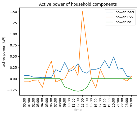
We can see how the controller uses the PV generated power to charge up the battery for future use. However, the controller only had access to inaccurate forecasts – therefore this is only the optimal control strategy conditioned on the available forecasting method.

Part 2: Safe Reinforcement Learning for Power System Control

We now want to control our power system using a neural network controller, which we train with reinforcement learning. A key challenge when using reinforcement learning is incorporating constraints of the system during both training and deployment. This is the core strength of CommonPower: Thanks to the symbolic modeling approach, we can automatically derive a safety shield that adjusts the control inputs proposed by the RL controller if necessary.

Training a Safe RL Agent

The first step is setting up an RL controller. In this case, we will use the Proximal Policy Optimization (PPO) algorithm from the StableBaselines3 (SB3) repository to train this agent. We have a specific controller class for this, the RLControllerSB3. The ObservationHandler defines how many forecasted values are integrated into the RL observation for each element that is obtained from data. Furthermore, we have to define a safety shield for the RL controller. We will use action projection here: each control input (action) suggested by the RL agent is adjusted as little as possible while still satisfying all constraints over the forecast horizon.

As previously mentioned, the safety shield obtains the safe action by solving a constrained optimization problem in each time step. The constraints are obtained from the symbolic model of the subsystem that is controlled by the RL agent – this is visualized in the figure below.

Figure 4: Safeguarding in CommonPower using symbolic modeling.

agent1 = RLControllerSB3(
    name='agent1',
    obs_handler=ObservationHandler(num_forecasts=13),
    safety_layer=ActionProjectionSafetyLayer(DistanceDependingPenalty(penalty_factor=0.0)),
    cost_callback=predicted_cost_callback
)
agent1.add_entity(n1)

/home/markgraf/repos/commonpower/commonpower/control/controllers.py:224: UserWarning: Node n0 already has a controller
  warnings.warn(f"Node {entity.id} already has a controller")
/home/markgraf/repos/commonpower/commonpower/control/controllers.py:232: UserWarning: Node n0.d00 already has a controller!
  warnings.warn(f"Node {child.id} already has a controller!")
/home/markgraf/repos/commonpower/commonpower/control/controllers.py:232: UserWarning: Node n0.r01 already has a controller!
  warnings.warn(f"Node {child.id} already has a controller!")
/home/markgraf/repos/commonpower/commonpower/control/controllers.py:232: UserWarning: Node n0.el02 already has a controller!
  warnings.warn(f"Node {child.id} already has a controller!")

<commonpower.control.controllers.RLControllerSB3 at 0x79dd0a96d630>

ℹ Adding the household to this controller provokes a warning since we are overriding the optimal controller from before. This can be helpful for debugging, but is desired in this case.

As explained in the section on safeguarding RL, we can add a penalty to the reward each time the safety shield has to intervene. This is what the penalty_factor refers to. We set it to 0 for now to show what happens if we do not incorporate any penalty.

Next, we want to define an episode_length for our system. The control horizon determines how many time steps the system will be simulated before it is reset. This is very useful for training an RL agent, since we can control how many consecutive time steps the system should be simulated. You can consider it an additional hyperparameter for training.

episode_length = 24  # [time steps] --> as the timedelta is 1 hour, this is 24h

Let us set up the configuration for the training algorithm, PPO. There are lots of hyperparameters you can tune for PPO. We will only modify some of them and use the default ones from StableBaselines3 for everything else.

# specify a seed for the random number generator used during training (It is common to train with ~5 different
# random seeds when you are, for example, testing a new safeguarding approach. For this notebook, one seed is enough.
# It will improve reproducibility of results.)
training_seed = 42

# set up configuration for the PPO algorithm
alg_config = SB3MetaConfig(
    total_steps=160*episode_length,
    seed=training_seed,
    algorithm=PPO,
    algorithm_config=SB3PPOConfig(
        n_steps=16*episode_length,
        batch_size=12,
        learning_rate=0.0008
    )  # otherwise default hyperparameters for PPO
)

We have to set up a logger to monitor our training process. We will use Tensorboard here, but CommonPower also supports Weights&Biases.

# set up logger
log_dir = './test_run/'
logger = TensorboardLogger(log_dir='./test_run/')
# specify the path where the model should be saved
model_path = "./saved_models/my_model"

Now we can start the training. We will use a different runner for that. Since CommonPower also supports multi-agent RL algorithms, we have a specific runner for single-agent algorithms from StableBaselines3. To adhere to the API of SB3, we use the SingleAgentWrapper which makes sure that the PPO algorithm can interact with our system (which is modeled as a OpenAI Gym environment).

runner = SingleAgentTrainer(
    sys=sys,
    wrapper=SingleAgentWrapper,
    alg_config=alg_config,
    horizon=forecast_horizon,
    episode_length=episode_length,
    logger = logger,
    save_path = model_path,
    seed = training_seed
)

We will visualize the training process using tensorboard. You might have to hit the refresh button to see the training.

%tensorboard --logdir test_run --reload_interval 1

Reusing TensorBoard on port 6006 (pid 1055779), started 2 days, 23:09:45 ago. (Use '!kill 1055779' to kill it.)

The procedure for training the RL agent is the same as for the deployment runner: You only have to call the run() method!

runner.run(fixed_start=test_day)

Using cpu device
Wrapping the env with a `Monitor` wrapper
Wrapping the env in a DummyVecEnv.
Logging to ./test_run/PPO_14

Go back to the tensorboard visualization to see how the return obtained by the agent rises (rollout/ep_rew_mean , i.e., the mean return over the last 100 episodes) . At the same time, the loss (loss, i.e., a weighted sum of the value loss, the policy gradient loss, and the entropy loss).

We also log some metrics that are specific for safe RL, namely the mean number of interventions by the safety layer (ep_corrections_mean), the mean penalty (ep_penalty_mean), and the mean reward without penalty (ep_rew_without_pen_mean). As you can see, the number of times that the safety layer has to correct the action of the RL agent increases over the training time.

❓ What could be the reason for this?

Benchmarking the RL Agent and the Optimal Controller

We now want to deploy the trained RL agent and compare its performance to the optimal controller.

rl_history = ModelHistory([sys])

rl_deployer = DeploymentRunner(
    sys=sys,
    horizon=forecast_horizon,
    history=rl_history,
    seed = eval_seed,
    alg_config=alg_config,
    wrapper=SingleAgentWrapper,
)

rl_deployer.run(n_steps=24, fixed_start=test_day)

  0%|          | 0/24 [00:00<?, ?it/s]100%|██████████| 24/24 [00:00<00:00, 29.08it/s]

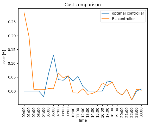
Let us plot the costs of the optimal controller and the RL controller:

oc_cost = oc_history.get_history_for_element(n1, 'cost')
rl_cost = rl_history.get_history_for_element(n1, 'cost')
plot_timeseries([oc_cost, rl_cost], ["optimal controller", "RL controller"], "Cost comparison", "time", "cost [€]", test_day_time_stamps)

Additionally, we want to have a look at the state of charge of the battery:

oc_soc = oc_history.get_history_for_element(e1, 'soc')
rl_soc = rl_history.get_history_for_element(e1, 'soc')
plot_timeseries([oc_soc, rl_soc], ["optimal controller", "RL controller"], "Comparison of State of Charge", "time", "state of charge [kWh]", test_day_time_stamps)

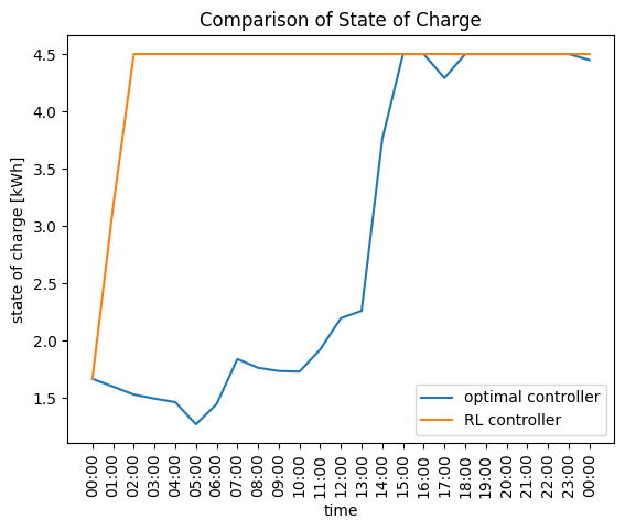
You can see that the agent has not learned a very good strategy, even though the learning curves indicate this. It tries to keep charging the battery even after it is fully charged, therefore the safety shield has to intervene.

We can also compare the cumulative cost over the day. However, we have to be careful: We cannot just compare controllers by tracking the realized cost until the last time step. This would neglect the fact that future anticipated costs affect the behavior during the time horizon we consider. Instead, we will use the function below, which computes the cost of the last time step as the accumulated cost over the forecast horizon. Since the projection is computed by the system’s “internal” solver, which is by definition optimal w.r.t. to the system’s cost function; this represents the “best case” cost (subject to the forecaster).

def get_adjusted_cost(hist: ModelHistory, sys: System):
    costs = hist.filter_for_entities(sys, False).filter_for_element_names("cost").history
    output = [c[1]["cost"][0] for c in costs]
    terminal_cost = np.sum(costs[-1][1]["cost"])
    output[-1] = terminal_cost
    return output

oc_cumulative_cost = get_adjusted_cost(oc_history, sys)
rl_cumulative_cost = get_adjusted_cost(rl_history, sys)
print(f"Cumulative cost using optimal controller: {round(sum(oc_cumulative_cost),2)} €")
print(f"Cumulative cost using RL controller: {round(sum(rl_cumulative_cost),2)} €")

Cumulative cost using optimal controller: 0.04 €
Cumulative cost using RL controller: 0.3 €

As you can see, the optimal controller significantly outperforms the RL controller. We will try to improve the performance of the RL controller by learning a policy that does not rely too much on the intervention of the safety shield.

Training a Safe RL Agent with a Penalty

With the first RL agent, we saw that the number of interventions of the safety shield increased during training. Because the agent was not aware of the safety shield, it thought that it was receiving high rewards for actions that were actually unsafe. This is why it learned a sub-optimal policy of always charging the battery.

To mitigate this, we will add a penalty to the reward each time the safety shield has to intervene. For this demonstration, we choose a penalty that is proportional to the magnitude of the necessary adjustment by setting the penalty_factor to 1.0.

agent2 = RLControllerSB3(
    name='agent2',
    obs_handler=ObservationHandler(num_forecasts=13),
    safety_layer=ActionProjectionSafetyLayer(DistanceDependingPenalty(penalty_factor=1.0)),
    cost_callback=predicted_cost_callback
)
agent2.add_entity(n1)

/home/markgraf/repos/commonpower/commonpower/control/controllers.py:224: UserWarning: Node n0 already has a controller
  warnings.warn(f"Node {entity.id} already has a controller")
/home/markgraf/repos/commonpower/commonpower/control/controllers.py:232: UserWarning: Node n0.d00 already has a controller!
  warnings.warn(f"Node {child.id} already has a controller!")
/home/markgraf/repos/commonpower/commonpower/control/controllers.py:232: UserWarning: Node n0.r01 already has a controller!
  warnings.warn(f"Node {child.id} already has a controller!")
/home/markgraf/repos/commonpower/commonpower/control/controllers.py:232: UserWarning: Node n0.el02 already has a controller!
  warnings.warn(f"Node {child.id} already has a controller!")

<commonpower.control.controllers.RLControllerSB3 at 0x79dcf2bb6560>

runner = SingleAgentTrainer(
    sys=sys,
    wrapper=SingleAgentWrapper,
    alg_config=alg_config,
    horizon=forecast_horizon,
    episode_length=episode_length,
    logger = logger,
    save_path = model_path,
    seed = training_seed
)

You can go back to the tensorboard visualization (and refresh it) to monitor this training run.

runner.run(fixed_start=test_day)

Using cpu device
Wrapping the env with a `Monitor` wrapper
Wrapping the env in a DummyVecEnv.
Logging to ./test_run/PPO_15

As you can see, the return obtained by the agent at the end of the training is lower – but the number of interventions from the safety layer has decreased significantly. Let’s see whether this has an effect during deployment.

rl_penalty_history = ModelHistory([sys])

rl_penalty_deployer = DeploymentRunner(
    sys=sys,
    horizon=forecast_horizon,
    history=rl_penalty_history,
    seed = eval_seed,
    alg_config=alg_config,
    wrapper=SingleAgentWrapper,
)

rl_penalty_deployer.run(n_steps=24, fixed_start=test_day)

  0%|          | 0/24 [00:00<?, ?it/s]100%|██████████| 24/24 [00:00<00:00, 29.89it/s]

rl_penalty_cost = rl_penalty_history.get_history_for_element(n1, 'cost')
rl_penalty_soc = rl_penalty_history.get_history_for_element(e1, 'soc')

rl_penalty_cumulative_cost = get_adjusted_cost(rl_penalty_history, sys)

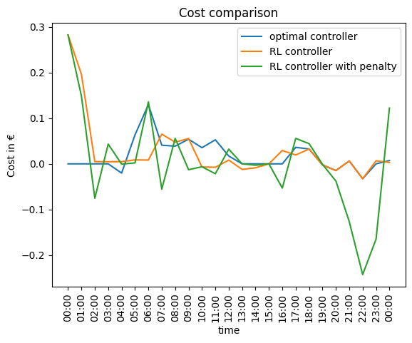
plot_timeseries([oc_cost, rl_cost, rl_penalty_cost], ["optimal controller", "RL controller", "RL controller with penalty"], "Cost comparison", "time", "Cost in €", test_day_time_stamps)

plot_timeseries([oc_soc, rl_soc, rl_penalty_soc], ["optimal controller", "RL controller", "RL_controller_with_penalty"], "Comparison of State of Charge", "time", "state of charge [kWh]", test_day_time_stamps)

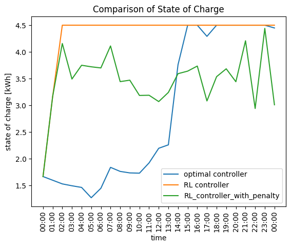
As you can see, the RL agent does no longer always try to overcharge the battery. Let us compare the cumulative cost of all three controllers.

print(f"Cumulative cost using optimal controller: {round(sum(oc_cumulative_cost),2)} €")
print(f"Cumulative cost using RL controller: {round(sum(rl_cumulative_cost),2)} €")
print(f"Cumulative cost using RL controller with penalty: {round(sum(rl_penalty_cumulative_cost),2)} €")

Cumulative cost using optimal controller: 0.04 €
Cumulative cost using RL controller: 0.3 €
Cumulative cost using RL controller with penalty: -0.28 €

The RL controller trained with the penalty actually outperforms the optimal controller. This is possible because we are using inaccurate forecasts of the load, the PV generation, and the electricity prices. However, this is only a very small example for one single day of a year (due to the time limit of this tutorial). We will next compare the performance of RL controllers trained on data from the entire year 2016 with both inaccurate and perfect forecasts.

Assessing the Impact of Forecast Accuracy

CommonPower offers an API for integrating different forecast strategies. We shortly want to demonstrate the impact of using a PersistenceForecaster vs. a PerfectKnowlegdeForecaster that will always predict the true values. An optimal controller that has access to perfect forecasts can serve as an lower bound for the minimum attainable cost.

To show the performance of different controllers over a longer time horizon (one week), we have pre-trained RL controllers on data from the entire year 2016. One agent was trained with perfect forecasts, the other one with the PersistenceForecaster. We will show you how to load pre-trained agents and then compare their performance against an optimal controller with the same forecast quality.

RL and Optimal Control with Persistence Forecasts

Our system is currently configured with the PersistenceForecaster. We will now simulate this system for one week (with time intervals of one hour) using an optimal controller.

evaluation_length = 7*episode_length  # one week

oc_persistence_controller = OptimalController("oc_persistent").add_entity(n1)

/home/markgraf/repos/commonpower/commonpower/control/controllers.py:224: UserWarning: Node n0 already has a controller
  warnings.warn(f"Node {entity.id} already has a controller")
/home/markgraf/repos/commonpower/commonpower/control/controllers.py:232: UserWarning: Node n0.d00 already has a controller!
  warnings.warn(f"Node {child.id} already has a controller!")
/home/markgraf/repos/commonpower/commonpower/control/controllers.py:232: UserWarning: Node n0.r01 already has a controller!
  warnings.warn(f"Node {child.id} already has a controller!")
/home/markgraf/repos/commonpower/commonpower/control/controllers.py:232: UserWarning: Node n0.el02 already has a controller!
  warnings.warn(f"Node {child.id} already has a controller!")

oc_persistence_history = ModelHistory([sys])

oc_persistence_runner = DeploymentRunner(
    sys=sys,
    horizon=forecast_horizon,
    history=oc_persistence_history,
    seed=eval_seed
)

oc_persistence_runner.set_start_time(test_day)  # starting from this day, we will simulate the system for one week
oc_persistence_runner.run(n_steps=evaluation_length)

  2%|▏         | 4/168 [00:00<00:04, 39.42it/s]100%|██████████| 168/168 [00:04<00:00, 37.16it/s]

# compute cost for benchmarking
oc_persistence_cost = oc_persistence_history.filter_for_entities(n1).filter_for_element_names(["cost"])
oc_persistence_soc = oc_persistence_history.filter_for_entities(e1).filter_for_element_names(["soc"])

oc_persistence_cumulative_cost = get_adjusted_cost(oc_persistence_history, sys)

Next, we want to load an agent that we pre-trained on data from the entire year 2016 (not just one day as done before). We will then simulate the system once more using this RL controller.

agent3 = RLControllerSB3(
    name="pretrained_agent",
    obs_handler=ObservationHandler(num_forecasts=13),
    safety_layer=ActionProjectionSafetyLayer(DistanceDependingPenalty(penalty_factor=1.0)),
    pretrained_policy_path = "saved_models/pretrained_models_ICLR/persistence_forecast_agent"
).add_entity(n1)

rl_persistence_history = ModelHistory([sys])

rl_persistence_deployer = DeploymentRunner(
    sys=sys,
    horizon=forecast_horizon,
    history=rl_persistence_history,
    seed = eval_seed,
    alg_config=alg_config,
    wrapper=SingleAgentWrapper,
)

rl_persistence_deployer.set_start_time(test_day)
rl_persistence_deployer.run(n_steps=evaluation_length)

100%|██████████| 168/168 [00:05<00:00, 32.01it/s]

# compute cost for benchmarking
rl_persistence_cost = rl_persistence_history.filter_for_entities(n1).filter_for_element_names(["cost"])
rl_persistence_soc = rl_persistence_history.filter_for_entities(e1).filter_for_element_names(["soc"])

rl_persistence_cumulative_cost = get_adjusted_cost(rl_persistence_history, sys)

We will compare the performance in the next subsection.

RL and Optimal Control with Perfect Forecasts

To switch to perfect predictions, we will simply create new data providers with a PerfectKnowledgeForecaster.

forecaster_2 = PerfectKnowledgeForecaster(frequency=forecast_frequency, horizon=forecast_horizon)

load_p_dp_perfect = DataProvider(p_load_ds, forecaster_2)
load_q_dp_perfect = DataProvider(q_load_ds, forecaster_2)
price_dp_perfect = DataProvider(buying_price_ds, forecaster_2)
selling_price_dp_perfect = DataProvider(selling_price_ds, forecaster_2)
pv_dp_perfect = DataProvider(pv_ds, forecaster_2)

We then have to add the new data providers to the respective components.

n1.clear_data_providers()
d1.clear_data_providers()
r1.clear_data_providers()

n1.add_data_provider(price_dp_perfect).add_data_provider(selling_price_dp_perfect)
d1.add_data_provider(load_p_dp_perfect).add_data_provider(load_q_dp_perfect)
r1.add_data_provider(pv_dp_perfect)

<commonpower.models.components.RenewableGen at 0x79dd11507880>

Now we can simulate the system for the same time span, once with an optimal controller and then with an RL controller that was pre-trained with perfect predictions.

oc_perfect_controller = OptimalController("oc_perfect").add_entity(n1)

oc_perfect_history = ModelHistory([sys])

oc_perfect_runner = DeploymentRunner(
    sys=sys,
    horizon=forecast_horizon,
    history=oc_perfect_history,
    seed = eval_seed
)

oc_perfect_runner.set_start_time(test_day)
oc_perfect_runner.run(n_steps=evaluation_length)

  0%|          | 0/168 [00:00<?, ?it/s]100%|██████████| 168/168 [00:04<00:00, 38.89it/s]

oc_perfect_cost = oc_perfect_history.filter_for_entities(n1).filter_for_element_names(["cost"])
oc_perfect_soc = oc_perfect_history.filter_for_entities(e1).filter_for_element_names(["soc"])

oc_perfect_cumulative_cost = get_adjusted_cost(oc_perfect_history, sys)

Let us load and deploy the RL controller with perfect forecasts:

agent4 = RLControllerSB3(
    name="pretrained_agent",
    obs_handler=ObservationHandler(num_forecasts=13),
    safety_layer=ActionProjectionSafetyLayer(DistanceDependingPenalty(penalty_factor=1.0)),
    pretrained_policy_path = "saved_models/pretrained_models_ICLR/perfect_forecast_agent"
).add_entity(n1)

rl_perfect_history = ModelHistory([sys])

rl_perfect_deployer = DeploymentRunner(
    sys=sys,
    horizon=forecast_horizon,
    history=rl_perfect_history,
    seed = eval_seed,
    alg_config=alg_config,
    wrapper=SingleAgentWrapper,
)

rl_perfect_deployer.set_start_time(test_day)
rl_perfect_deployer.run(n_steps=evaluation_length)

  0%|          | 0/168 [00:00<?, ?it/s]100%|██████████| 168/168 [00:04<00:00, 33.97it/s]

rl_perfect_cost = rl_perfect_history.filter_for_entities(n1).filter_for_element_names(["cost"])
rl_perfect_soc = rl_perfect_history.filter_for_entities(e1).filter_for_element_names(["soc"])

rl_perfect_cumulative_cost = get_adjusted_cost(rl_perfect_history, sys)

Now we can compare the cumulative cost of all controllers:

print(f"Cumulative cost using optimal controller and perfect forecasts: {round(sum(oc_perfect_cumulative_cost),2)} €")
print(f"Cumulative cost using RL controller and perfect forecasts: {round(sum(rl_perfect_cumulative_cost),2)} €")
print(f"Cumulative cost using optimal controller and persistence forecasts: {round(sum(oc_persistence_cumulative_cost),2)} €")
print(f"Cumulative cost using RL controller and persistence forecasts: {round(sum(rl_persistence_cumulative_cost),2)} €")

Cumulative cost using optimal controller and perfect forecasts: 6.3 €
Cumulative cost using RL controller and perfect forecasts: 9.62 €
Cumulative cost using optimal controller and persistence forecasts: 8.54 €
Cumulative cost using RL controller and persistence forecasts: 9.44 €

You can see that the performance of the RL controller and optimal controller are much closer if we use imperfect forecasts. Of course, we would need to perform a more thorough evaluation over a longer time horizon and with different random seeds during training to make this a valid claim. However, in this tutorial, we mainly wanted to showcase that the choice of a forecasting method has a huge impact – and that the potential of using RL controllers unfolds if you do not have good forecasts available!

Part 3: More Advanced Capabilities of CommonPower

So far, we have considered a very simple use case to explain the core concepts of CommonPower. Now, we want to show you a few more advanced capabilities.

First of all, CommonPower also allows you to simulate power grids – not just single buildings. You can import network topologies from pandapower and modify them if necessary.

Another possibility is implementing your custom entities – this could for example be an electric vehicle, a heat pump with a thermal storage (we have a simplified model, but this could be extended), or even a different formulation for power flow equations like LinDistFlow.

More Realistic Power Grid Modeling

CommonPower comes with a utility that enables importing power grid topologies from the pandapower library, the PandaPowerImporter. To conveniently add Components to nodes within the imported grid, we can define a Factory which allows defining component templates and encapsulates options for randomization.

Furthermore, we can use a more realistic power flow model based on the DC power flow equations.

from numpy.random import uniform

import pandapower.networks as pn

from commonpower.extensions.factories import Factory, Sampler
from commonpower.extensions.network_import import PandaPowerImporter
from commonpower.models.powerflow import DCPowerFlowModel

def spawn_sys(
        load_dp,
        pv_dp,
        price_dp
    ) -> System:

    factory = Factory()

    factory.set_bus_template(Bus, meta_config={})  # use default Bus config

    # add components to factory

    # Every node has a load component
    factory.add_component_template(Load, probability=1., data_providers=[load_dp])

    # A node has a PV component with a probability of 70%
    factory.add_component_template(
      RenewableGen,
      probability=.7,
      meta_config={
        "p": Sampler(uniform, low=[-10, 0], high=[-3, 0]),  # If a PV component is added, it will sample its maximum generation power uniformly from [-10, -3] kW
        #"q": Sampler(uniform, low=[0, 0], high=[0, 0])
      },
      data_providers=[pv_dp]
    )

    # initialize system
    net = pn.create_kerber_landnetz_kabel_2()
    sys = PandaPowerImporter().import_net(net=net, power_flow_model=DCPowerFlowModel(), node_factory=factory, restrict_factory_to="loadbus")

    trading_node = TradingBusLinear("TradingBus", {}).add_data_provider(price_dp)

    #### some specific adjustments for this grid

    # set node 1 (main_busbar) as external grid connection, i.e. trading node
    sys.add_node(trading_node, at_index=1)

    # update the respective lines
    sys.lines[0].src = trading_node
    sys.lines[24].src = trading_node

    # remove line from ext to main busbar
    sys.lines.pop(-1)
    # remove node 0
    sys.nodes.pop(0)

    return sys

sys = spawn_sys(load_p_dp, pv_dp, price_dp)
sys.pprint()

SYSTEM OVERVIEW

Nodes:
    (TradingBusLinear): TradingBus
    (Bus): MUF_1_1
    (Bus): loadbus_1_1
       (Load): Load
       (RenewableGen): RenewableGen
    (Bus): KV_1_2
    (Bus): loadbus_1_2
       (Load): Load
    (Bus): MUF_1_3
    (Bus): loadbus_1_3
       (Load): Load
       (RenewableGen): RenewableGen
    (Bus): KV_1_4
    (Bus): loadbus_1_4
       (Load): Load
       (RenewableGen): RenewableGen
    (Bus): MUF_1_5
    (Bus): loadbus_1_5
       (Load): Load
       (RenewableGen): RenewableGen
    (Bus): KV_1_6
    (Bus): loadbus_1_6
       (Load): Load
       (RenewableGen): RenewableGen
    (Bus): MUF_1_7
    (Bus): loadbus_1_7
       (Load): Load
       (RenewableGen): RenewableGen
    (Bus): KV_1_8
    (Bus): loadbus_1_8
       (Load): Load
    (Bus): MUF_1_9
    (Bus): loadbus_1_9
       (Load): Load
       (RenewableGen): RenewableGen
    (Bus): KV_1_10
    (Bus): loadbus_1_10
       (Load): Load
       (RenewableGen): RenewableGen
    (Bus): MUF_1_11
    (Bus): loadbus_1_11
       (Load): Load
       (RenewableGen): RenewableGen
    (Bus): KV_1_12
    (Bus): loadbus_1_12
       (Load): Load
    (Bus): MUF_2_1
    (Bus): loadbus_2_1
       (Load): Load
       (RenewableGen): RenewableGen
    (Bus): KV_2_2
    (Bus): loadbus_2_2
       (Load): Load

Lines:
   lb_3435f: TradingBus -- MUF_1_1
   lb_7fa84: MUF_1_1 -- loadbus_1_1
   lb_06b6e: MUF_1_1 -- KV_1_2
   lb_6ef73: KV_1_2 -- loadbus_1_2
   lb_d0f92: KV_1_2 -- MUF_1_3
   lb_8f185: MUF_1_3 -- loadbus_1_3
   lb_5d390: MUF_1_3 -- KV_1_4
   lb_c7645: KV_1_4 -- loadbus_1_4
   lb_51b7a: KV_1_4 -- MUF_1_5
   lb_24d43: MUF_1_5 -- loadbus_1_5
   lb_470c8: MUF_1_5 -- KV_1_6
   lb_e3c18: KV_1_6 -- loadbus_1_6
   lb_40deb: KV_1_6 -- MUF_1_7
   lb_43b51: MUF_1_7 -- loadbus_1_7
   lb_00e8a: MUF_1_7 -- KV_1_8
   lb_02b86: KV_1_8 -- loadbus_1_8
   lb_6b3dd: KV_1_8 -- MUF_1_9
   lb_6e538: MUF_1_9 -- loadbus_1_9
   lb_54eb2: MUF_1_9 -- KV_1_10
   lb_553d7: KV_1_10 -- loadbus_1_10
   lb_941fc: KV_1_10 -- MUF_1_11
   lb_a096e: MUF_1_11 -- loadbus_1_11
   lb_65d4d: MUF_1_11 -- KV_1_12
   lb_68d8d: KV_1_12 -- loadbus_1_12
   lb_5d03a: TradingBus -- MUF_2_1
   lb_64cd5: MUF_2_1 -- loadbus_2_1
   lb_c435d: MUF_2_1 -- KV_2_2
   lb_98fad: KV_2_2 -- loadbus_2_2

Creating Your Own Component Models

CommonPower has a pre-defined linear model of an ESS: ESSLinear. We will extend this component to include

• a state of health (SOH), and

• charging efficiencies and self-discharge.

The SOH is included as an (observable) variable and governs the maximum and minimum battery capacity. The SOH evolves according to a difference equation that is included in the symbolic component model.

This symbolic model is used by the safety layer and the built-in optimal controller. However, components implement an _update_state() method that we can overwrite to simulate different or more realistic dynamics compared to the symbolic model. We can also add some parameters for the “true” dynamics to the __init__() method of the component. We use this mechanism to include charging efficiency and self-discharge in the state update.

class ESSTrueDynamicsSOH(ESSLinear):

  @classmethod
  def _get_model_elements(cls) -> List[ModelElement]:
    """
    All the elements defined here are observable and are assumed to require configuration.
    """
    model_elements = [
        ModelElement("p", et.INPUT, "active power"),
        ModelElement("q", et.VAR, "reactive power"),
        ModelElement("soc", et.STATE, "state of charge (absolute)", pyo.NonNegativeReals),
        ModelElement("soh", et.STATE, "state of health (relative)", bounds=(0,1)),  # this is new
    ]

    return model_elements

  def __init__(
    self,
    name: str,
    config: dict = {},
    charge_efficiency: float = 0.95,
    self_discharge: float = 0.99
  ):

    super().__init__(name, config)

    self.etac = charge_efficiency
    self.etas = self_discharge

  def _get_additional_constraints(self) -> List[ModelElement]:
    """
    This method can be used to add additional input/state constraints.
    We can also add additional (helper) variables.
    Everything that is defined here is not exposed for user configuration.
    """

    # We define a binary indicator variable which tells us if the battery is being charged or discharged.
    # This indicator will be used in the dynamics equation to update the SOH.
    # To facilitate the creation of such indicator variables and corresponding constraints, we built a utility: The MIPExpressionBuilder

    mb = MIPExpressionBuilder(self)
    # We want to model: p_ec = 1 if p>=0 else 0
    # The expression builder automatically generates all corresponding constraints as model elements (based on the big-M method)
    mb.from_geq("p", 0, "p_ec")

    # We add contraints limiting the capacity depending on the current SOH
    # soc <= soh * max(soc)
    # soc >= soh * min(soc)

    def soh_soc_upper_f(model, t):
      return (
        self.get_pyomo_element("soc", model)[t]
        <= self.get_pyomo_element("soh", model)[t] * self.get_pyomo_element("soc", model)[t].ub
      )

    def soh_soc_lower_f(model, t):
      return (
        self.get_pyomo_element("soc", model)[t]
        >= self.get_pyomo_element("soh", model)[t] * self.get_pyomo_element("soc", model)[t].lb
      )

    c_soh_soc_upper = ModelElement(
      "c_soh_soc_upper",
      et.CONSTRAINT,
      "contraint limiting the max capacity depending on the current SOH",
      expr=soh_soc_upper_f,
      indexed=True,
    )

    c_soh_soc_lower = ModelElement(
      "c_soh_soc_lower",
      et.CONSTRAINT,
      "contraint limiting the min capacity depending on the current SOH",
      expr=soh_soc_lower_f,
      indexed=True,
    )

    return mb.model_elements + [c_soh_soc_upper, c_soh_soc_lower]

  def _get_dynamic_fcn(self) -> List[ModelElement]:
      """
      This is the already defined dynamics equation: soc_{t+1} = soc_{t} + p_t
      We now add: soh_{t+1} = soh_t - 1e-7 * abs(p_t)
      This encodes that we loose 1% capacity after 100,000 kWh of charging/discharging.
      """

      def soc_dynamics_f(model, t):
        # p > 0 is charging
        if t == self.horizon:
          return Constraint.Skip
        else:
          return (
            self.get_pyomo_element("soc", model)[t] + self.get_pyomo_element("p", model)[t] * self.tau
            == self.get_pyomo_element("soc", model)[t + 1]
          )

      def soh_dynamics_f(model, t):
        # p > 0 is charging
        if t == self.horizon:
          return Constraint.Skip
        else:
          return (
            self.get_pyomo_element("soh", model)[t]
            - (
                (  # charging
                  self.get_pyomo_element("p", model)[t] * self.get_pyomo_element("p_ec", model)[t]
                )
                + (  # discharging
                  - self.get_pyomo_element("p", model)[t] * (1 - self.get_pyomo_element("p_ec", model)[t])
                )
            ) * 1e-7 * self.tau
            == self.get_pyomo_element("soh", model)[t + 1]
          )

      soc_dyn = ModelElement("soc_dynamics", et.CONSTRAINT, "dynamics of SOC", expr=soc_dynamics_f)
      soh_dyn = ModelElement("soh_dynamics", et.CONSTRAINT, "dynamics of SOH", expr=soh_dynamics_f)

      return [soc_dyn, soh_dyn]

  def _update_state(self):
    """
    The default method simply uses the solved system model from the previous time step to update the states:

      for el in [el for el in self.model_elements if el.type == ElementTypes.STATE]:
        values = self.get_value(self.instance, el.name)
        for t in range(0, self.horizon):
            self.set_value(
                self.instance,
                el.name,
                values[t + 1],
                idx=t,
                fix_value=(t == 0),
            )

    We now change this to include the charging efficiency and self-discharge:
    soc_{t+1} = etas * soc_t + etac * p_t, if p_t >= 0 (charging)
    soc_{t+1} = etas * soc_t + 1/etac * p_t, if p_t < 0 (discharging)
    """

    soc_values = self.get_value(self.instance, "soc")
    p_values = self.get_value(self.instance, "p")

    for t in range(0, self.horizon):
        new_soc = self.self_dicharge * soc_values[t] + (self.charge_efficiency if p_values[t] >= 0 else 1/self.charge_efficiency) * p_values[t]
        self.set_value(
            self.instance,
            "soc",
            new_soc,
            idx=t,
            fix_value=(t == 0),  # this will be the initial state of the next iteration and must not be treated as a variable by the solver.
        )

If we now used ESSTrueDynamicsSOH, the safety layer would establish safety based on the nominal/symbolic model. This could lead to an over-discharge as efficiencies were not considered. Countermeasures would be to include disturbances/efficiencies in the symbolic model (see e.g. the pre-defined ESS model) or to adjust the component’s state limits.

With the features introduced in this section, you are able to create your own benchmarks and test different safe RL algorithms on them! We also have an interface for multi-agent RL – but this is not within the scope of this tutorial. Make sure to check out our repository for more tutorials!

Discussion

We introduced how to use the CommonPower toolbox to

• create benchmarks for power system control in a modular fashion,

• train safe RL agents to solve these problems, and

• incorporate different forecasting methods to generate predictions of quantities such as load, generation, or electricity prices, which are observed by RL agents.

Thanks for completing this tutorial! Let us summarize what we learned, discuss a few limitations, and consider some potential next steps.

Lessons Learned

• If there are any constraints present in the environment that an RL agent interacts with, you have to be careful: Simply adjusting the actions chosen by the RL agent may lead to suboptimal policies.

• One option to mitigate this effect is to use a penalty each time the action of the RL agent has to be adjusted. This can improve the performance of the safe RL agent.

• Another factor that has a noticable impact on the performace of an RL agent is the forecasting method that is used to generate the observations the agent receives. This is often overlooked in tools that aim at benchmarking RL for power system control!

Limitations

• We have used a very simple example to showcase the capabilities of the CommonPower toolbox. To make valid claims on how well RL agents trained with different forecasters and safety shield configurations perform, we would have to conduct multiple training runs with different random seeds and evaluate them over a separate test set.

• The interplay of different RL algorithms and safeguarding options for power system control needs to be studied in more detail. For example, action projection might hinder exploration since it always outputs the action closest to the unsafe action – which in many situations will be the minimum or maximum of the admissable actions.

Next Steps

• Try running the examples presented here on different random seeds. Is the training robust?

• Evaluate the pre-trained agents on a longer time horizon – for example the entire year!

• Extend the simplified use case – for example by adding a heat pump to the building. You can use our HeatPumpWithoutStorageButCOP – or implement your own heat pump model!

• We encourage you to implement your own benchmarking problems in CommonPower and test different safeguarding options for RL algorithms! If you want to model a multi-agent control task, consider our tutorial on multi-agent RL with CommonPower.

• CommonPower has only very simple forecasting methods implemented so far. We would be happy if you want to test your advanced forecasting method in an RL setting. You can build on top of our Forecaster class to adhere to our API.

Related Ressources

The following existing CCAI tutorials are related to our work and can provide you with more insights into RL for building management.

• BOPTEST tutorial: Introduction to controlling the heating, ventilation, and cooling (HVAC) system of a building using RL

• CityLearn tutorial: Introduction to multi-agent RL for building management systems

• Load forecasting tutorial: Introduction to household load forecasting using machine learning

References

(Brunke et al., 2022): Brunke, Lukas, et al. “Safe learning in robotics: From learning-based control to safe reinforcement learning.” Annual Review of Control, Robotics, and Autonomous Systems 5 (2022): 411-444.

(Krasowski et al., 2022): Krasowski, Hanna, et al. “Provably safe reinforcement learning: A theoretical and experimental comparison.” arXiv preprint arXiv:2205.06750 (2022).

(Sutton et al., 2018): Sutton, Richard S., and Andrew G. Barto. Reinforcement learning: An introduction. MIT press, 2018.

(Yu et al., 2022): Yu, Chao, et al. “The surprising effectiveness of ppo in cooperative multi-agent games.” Advances in Neural Information Processing Systems 35 (2022): 24611-24624.